Why IoT ML projects hit memory limits fast
Teams usually discover the memory problem late: the prototype works on a dev board with plenty of headroom, then fails on the production MCU once you add the real sensor stack, radios, logging, and power management. Even a “small” model can be large relative to 128–512 KB of RAM and a few megabytes (or less) of flash, especially when frameworks bring along runtimes, operators, and alignment overhead.
Memory pressure also spikes during inference, not just from the stored weights. Feature windows, intermediate tensors, ring buffers, and DMA-friendly sensor buffers can create short RAM peaks that exceed the budget even if the average looks fine. Add OTA update safety margins and you may need to reserve extra flash for dual images, which turns “it fits” into “it doesn’t ship.”
Where the memory goes: model, runtime, and data buffers
A useful way to debug “it doesn’t fit” is to split usage into three buckets: the model in flash, the ML runtime in flash/RAM, and the data buffers in RAM. The model is mostly weights plus a small graph or metadata, but the runtime often costs more than expected: operator kernels, lookup tables, scratch arenas, and any math libraries pulled in by a single layer type. That overhead is why two models with similar accuracy can have very different footprints on the same MCU.
RAM pain usually comes from buffers you didn’t think of as “ML.” Sensor drivers prefer chunky DMA buffers; feature extraction wants windows (e.g., 1–3 seconds of audio or vibration); inference needs activation tensors, sometimes multiple at once. These buffers stack, and alignment can add padding. You can reduce peaks, but it may raise latency, constrain sampling rates, or complicate OTA testing because memory maps become tighter and less flexible.
What makes TinyML different from “edge ML” claims
A lot of “edge ML” marketing still assumes a relatively capable edge: Linux-class gateways, NPUs, or at least enough RAM to carry a full framework and float32 models. TinyML is the stricter version: microcontrollers that spend most of their time asleep, wake up for a short burst of sensing and inference, and run without an OS (or with a very small RTOS) inside tens to hundreds of KB of RAM.
You treat the model as one component in a tight memory map, and you design the feature pipeline to avoid RAM spikes. The payoff is less radio use and lower latency because you don’t stream raw data to the cloud. The cost is real: you may accept lower accuracy, narrower operating conditions, more effort to quantize and validate, and a more careful update story (tooling, reproducible builds, and regression tests) because tiny changes can break the fit.
Model choices that shrink flash without killing accuracy
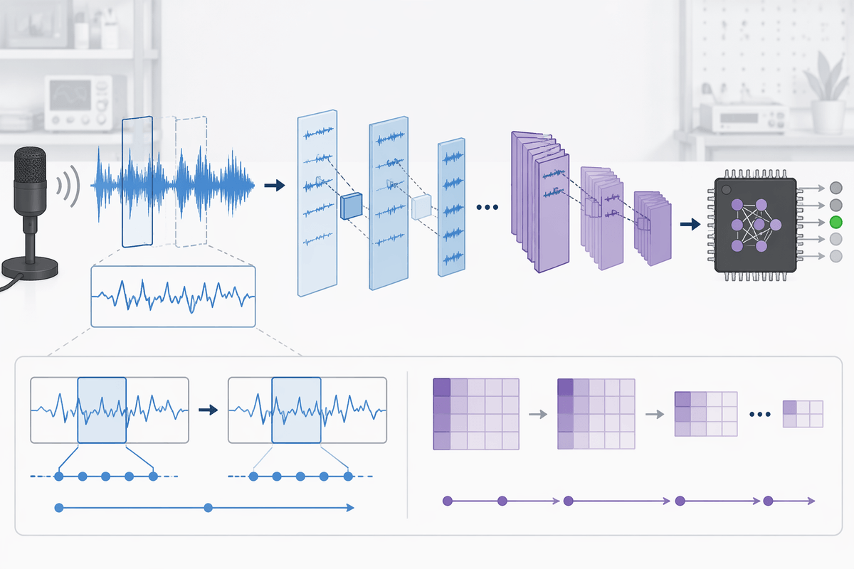
The familiar failure mode is choosing a “standard” architecture because it’s easy to train, then discovering it drags in heavy kernels and weight storage that dominate flash. On tiny MCUs, simpler layer types often win twice: fewer parameters and a smaller runtime surface area. Depthwise-separable convs, small 1D convs for time-series, and compact keyword-spotting CNNs can replace larger 2D conv stacks or LSTMs with similar on-device accuracy once you tune the receptive field and stride for your sampling rate.
Another lever is to pick models that naturally tolerate aggressive pruning of capacity. For many sensing tasks, the tail of channels and hidden units contributes little beyond a point. Narrowing early layers can cut flash substantially because those layers feed most activations and weights, while carefully keeping later layers wide enough to preserve class separation. Distillation can also help: train a larger “teacher” model offline, then train a smaller “student” that matches its outputs, often keeping accuracy higher than a small model trained from scratch.
Nonstandard architectures may reduce flash, but they can complicate deployment if your runtime doesn’t have optimized kernels, and they can make future model iterations slower because the team has to retrain, re-benchmark, and re-validate memory maps on every change.
Quantization and integer inference: biggest wins for tiny devices
The most reliable way to free flash and RAM on a microcontroller is to stop treating float32 as the default. Quantization replaces 32-bit weights (and often activations) with 8-bit integers, typically cutting weight storage by about 4× and shrinking activation buffers that drive RAM peaks. In practice, this is often the difference between “barely fits” and “leaves room for the rest of the firmware,” especially once you account for OTA slots and non-ML code.
Integer inference also simplifies the compute path. Many MCUs have fast 8-bit MAC instructions, and integer kernels avoid pulling in heavier floating-point math. The trade-off is that you’re now depending on calibration quality and operator support. Post-training quantization can be quick, but it can fail badly on models with sensitive layers or odd activation ranges. Quantization-aware training usually recovers accuracy, but it adds training time, requires tighter version control on preprocessing, and forces you to validate the full pipeline end-to-end on real sensor data, not just a held-out dataset.
Tooling friction is real: missing int8 kernels for one layer can silently force a float fallback, ballooning both flash and RAM. Treat “fully integer” as a hard requirement, and budget time to inspect the compiled operator list before you declare the memory problem solved.
Reducing RAM peaks: streaming features and smarter buffers
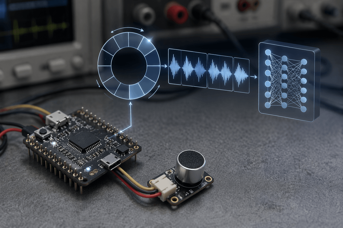
The moment RAM blows up is usually when you try to “batch” reality: collect a big sensor window, compute a big feature matrix, then run inference on top. On a 256 KB RAM MCU, a few seconds of audio, a 2D spectrogram, and a couple of scratch buffers can exceed budget even if the int8 model is tiny. The alternative is to stream: keep a small ring buffer of raw samples, compute features incrementally (frame-by-frame), and feed the model in chunks so you never materialize the full window in RAM.
Start by treating buffers as first-class design objects. Reuse memory aggressively: let feature extraction write into the same arena used for inference activations, and prefer in-place ops and fixed-size workspaces over “convenient” intermediate arrays. Make DMA buffers just large enough for timing jitter, not large enough to feel safe. If your runtime supports it, pre-plan tensor lifetimes so scratch is shared across layers instead of reserved per op.
Streaming pipelines are harder to debug, off-by-one errors show up as accuracy drops, and tighter buffers reduce tolerance to sensor stalls or RTOS scheduling delays. You often trade RAM headroom for more careful testing under worst-case timing and temperature.
A practical checklist to ship TinyML within memory budgets
A typical shipping failure is treating “the model fits” as the milestone, then discovering the integrated firmware doesn’t. Lock a memory budget early (flash for code + weights + OTA slots, RAM for stacks + DMA + arenas), and make it a CI gate with map files and peak-RAM measurements. Require fully int8 operators (no float fallbacks), and treat preprocessing as part of the model: version it, unit-test it, and profile its buffers. Stream features to avoid materializing big windows, and explicitly plan buffer reuse across sensing, DSP, and inference. Finally, test worst-case timing—radio on, logs enabled, cold battery—because that’s when RAM peaks and latency surprises appear.