When pattern recognition hits a ceiling with standard deep learning
Teams often start with a strong baseline: a CNN for images, a transformer for sequences, maybe a 3D model for point clouds. Early gains are fast, then progress slows. You add more data, widen the network, tune longer, and accuracy barely moves. The model is still “seeing” patterns, but it is relearning the same idea under many views—rotations, translations, different sensor orientations, or reordered parts of a graph—because the structure of the problem isn’t built into the model.
This ceiling shows up when the task depends on relationships more than raw texture: molecules where bond geometry matters, industrial vision where parts appear at arbitrary angles, or signals where phase shifts shouldn’t change the class. Standard deep learning can handle these cases, but it often pays a steep sample and compute cost to do it. That cost becomes a product constraint: longer training cycles, bigger labeling budgets, and improvements that are hard to justify beyond a certain point.
What “Geometric AI” actually adds beyond pixels and tokens
Picture a camera-based inspection line where the same part shows up at unpredictable angles, or a fraud model where the “shape” of transactions matters more than any single field. Geometric AI is a family of models that treats the data as something with structure—nodes and edges, points and orientations, surfaces and symmetries—rather than as a flat grid of pixels or a simple sequence of tokens. Instead of hoping the network learns these relationships from examples, you represent them explicitly and train the model to operate on them directly.
In practice, that often means building a graph from your entities and interactions, using point clouds with local neighborhoods, or adding orientation-aware features so a rotation is handled consistently. The upside is fewer redundant examples to learn “the same thing” in different poses, which can translate to better accuracy and stability under distribution shift. You need careful data-to-geometry preprocessing, more design choices to validate, and debugging can be harder than with standard CNN/transformer pipelines.
Why respecting symmetry and invariance can raise accuracy
A familiar failure case is when a classifier changes its mind because the input is “the same” in any reasonable sense, but not identical in raw coordinates. A bolt rotated 30 degrees, a LiDAR scan taken from a different heading, a protein conformation shifted in space, or a graph with nodes renumbered can all look different to a standard model. If the task label should not change under that transformation, forcing the model to relearn it from data wastes capacity and often shows up as brittle edge cases in production.
Geometric models bake in invariance (outputs stay the same) or equivariance (outputs transform predictably) to symmetries like translation, rotation, reflection, and permutation. That reduces the hypothesis space: the model is discouraged from using accidental cues such as absolute position or arbitrary node order, and pushed toward features that remain meaningful across views. The practical payoff is often higher accuracy with less data, plus better calibration when sensors, orientations, or interaction patterns drift.
You must choose the right symmetry to enforce; get it wrong and you can remove real signal (for example, “left vs. right” parts or absolute location on a wafer). Equivariant layers can be slower and more memory-hungry, so the gain has to justify added latency and engineering effort.
Choosing the right geometric representation for your data
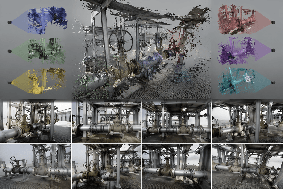
A practical way to decide is to start from what stays consistent when the input changes. If objects move around but keep their shape, you likely need coordinates plus a notion of local neighborhood (points, patches, or keypoints), not just an image grid. If the problem is “who interacts with whom,” as in molecules, power networks, or transaction flows, a graph is usually the honest representation—even if the raw data arrives as tables.
Representation choices also lock in what the model can easily learn. Point clouds preserve metric distance and orientation but require choices about sampling density and neighbor radius. Graphs make connectivity explicit, but edge definitions (k-NN vs. physical bonds vs. learned edges) can dominate results. Meshes and surfaces help when curvature matters, but they raise preprocessing complexity and failure modes around holes, noise, and topology changes.
One useful constraint check is operational: can you generate the geometry reliably at scale, and can you keep it stable across sensors and sites? If geometry construction is brittle, the “geometric” advantage can turn into data drift, slower inference, and harder debugging than a simpler baseline.
Model options: GNNs, equivariant nets, and hybrid pipelines
A common decision point is whether you need the model to reason over relationships, over physical space, or both. Graph neural networks (GNNs) are the straightforward choice when edges are meaningful: molecular bonds, network links, supply-chain flows, or “who-touched-what” event graphs. They aggregate information across neighbors, which often improves accuracy on tasks where context matters more than any single node’s features. The catch is that your edge and feature design can dominate outcomes; a “wrong but plausible” graph can quietly cap performance.
Equivariant networks focus on consistent behavior under transformations such as rotation and translation, which is valuable for 3D vision, robotics, protein structure, and orientation-heavy inspection. They can reduce the need for heavy augmentation, but they tend to cost more in latency and memory, and you have to pick the symmetry group that matches reality.
Hybrid pipelines are common in products: a CNN or transformer extracts local features, then a GNN or equivariant head enforces structure for the final decision. This often wins when you need incremental gains without rebuilding everything, but integration adds plumbing: multiple data formats, more hyperparameters, and more places for silent preprocessing bugs.
Training and evaluation gotchas that hide real gains
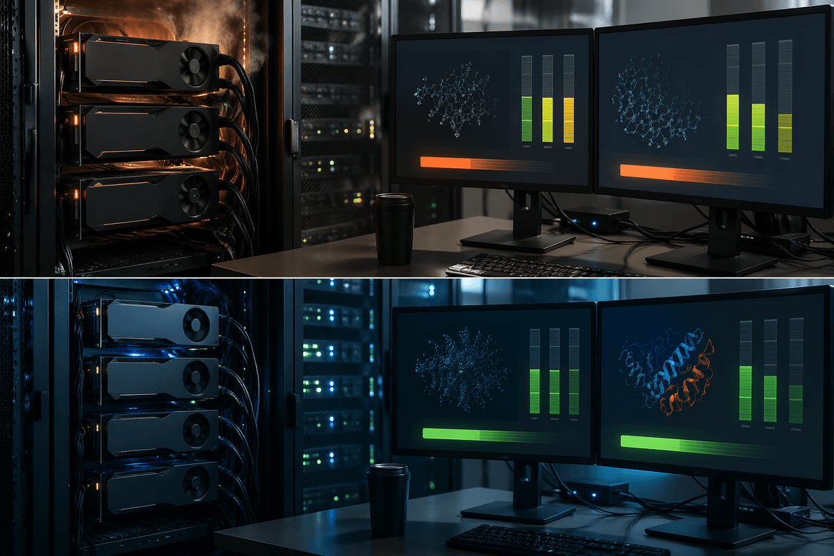
A familiar frustration is seeing a geometric model look “no better” than a strong CNN/transformer, even when the task should benefit from symmetry. Often the issue is evaluation leakage or mismatch. If your train/test split shares near-duplicate scenes (same part, same scan, different crop), both models look great and the geometric advantage disappears. If the split is too harsh (new factories, new sensors, new graph construction rules), you may be measuring pipeline drift, not model capability.
Augmentation is another trap. Teams sometimes keep heavy rotation/translation augmentation while also enforcing equivariance, effectively training the model to solve an already-solved invariance problem, wasting capacity and compute. At the other extreme, removing augmentation entirely can hurt because real data includes non-symmetric effects (occlusion, lighting, missing nodes, irregular sampling).
Finally, compare wall-clock and stability, not just top-1 accuracy. Equivariant layers can be slower and more memory-hungry, and geometric preprocessing can fail silently (bad edges, wrong units, inconsistent coordinate frames). Track these as first-class metrics or the “gain” won’t survive production.
A practical adoption checklist for boosting recognition accuracy
If you’re considering a pilot, start by writing down the transformations that should not change the answer (rotation, translation, node reindexing) and the ones that should (left/right, absolute location, orientation). Convert a small but representative slice of data into the geometric form you’d actually ship—graph edges, coordinate frames, units, neighborhood rules—and validate it with simple visual/logic checks before modeling.
Run an apples-to-apples baseline: same split, same label policy, and a test set that reflects real shift (new sites, poses, or interaction patterns). Measure accuracy plus latency, memory, and preprocessing failure rate. Plan for added engineering cost: geometry construction, debugging tools, and monitoring for drift in edges or coordinate conventions. Only scale if the gain persists across at least two independent slices of production-like data.